Understanding Hinton

Part of
Understanding Hinton’s Capsule Networks Series:

Part I: Intuition
(you are reading it now)
Part II: How
Capsules Work
Part III: Dynamic
Routing Between Capsules
Part IV: CapsNet Architecture

Quick announcement about our new publication AI³.
We are getting the best writers together to talk about the
Theory, Practice, and Business of AI and machine learning. Follow it to
stay up to date on the latest trends.

1. Introduction

Last week, Geoffrey Hinton and his team published two papers that
introduced a completely new type of neural network based on so-called
capsules. In addition to that, the team published an algorithm,
called dynamic routing between capsules, that allows to train
such a network.

Geoffrey Hinton has spent decades thinking about capsules. Source.

For everyone in the deep learning community, this is huge news, and
for several reasons. First of all, Hinton is one of the founders of deep
learning and an inventor of numerous models and algorithms that are
widely used today. Secondly, these papers introduce something completely
new, and this is very exciting because it will most likely stimulate
additional wave of research and very cool applications.

In this post, I will explain why this new architecture is so
important, as well as intuition behind it. In the following posts I will
dive into technical details.

However, before talking about capsules, we need to have a look at
CNNs, which are the workhorse of today’s deep learning.

Architecture of CapsNet from the original paper.

2. CNNs Have Important
Drawbacks

CNNs (convolutional
neural networks) are awesome. They are one of the reasons deep
learning is so popular today. They can do amazing
things that people used to think computers would not be capable of
doing for a long, long time. Nonetheless, they have their limits and
they have fundamental drawbacks.

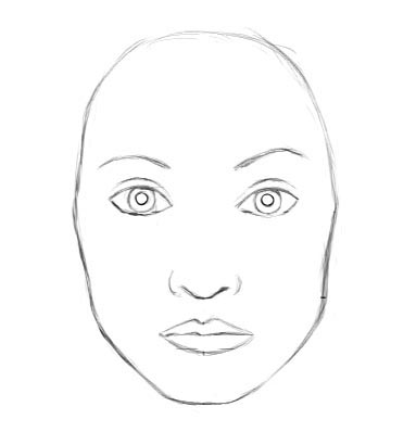
Let us consider a very simple and non-technical example. Imagine a
face. What are the components? We have the face oval, two eyes, a nose
and a mouth. For a CNN, a mere presence of these objects can be a very
strong indicator to consider that there is a face in the image.
Orientational and relative spatial relationships between these
components are not very important to a CNN.

To a CNN, both pictures are similar, since they both contain similar
elements. Source.

How do CNNs work? The main component of a CNN is a convolutional
layer. Its job is to detect important features in the image pixels.
Layers that are deeper (closer to the input) will learn to detect simple
features such as edges and
color gradients, whereas higher layers will combine simple features
into more complex features. Finally, dense layers at the top of the
network will combine very high level features and produce classification
predictions.

An important thing to understand is that higher-level features
combine lower-level features as a weighted sum: activations of a
preceding layer are multiplied by the following layer neuron’s weights
and added, before being passed to activation nonlinearity. Nowhere in
this setup there is pose(translational and rotational)
relationship between simpler features that make up a higher level
feature. CNN approach to solve this issue is to use max pooling or
successive convolutional layers that reduce spacial size of the data
flowing through the network and therefore increase the “field of view”
of higher layer’s neurons, thus allowing them to detect higher order
features in a larger region of the input image. Max pooling is a crutch
that made convolutional networks work surprisingly well, achieving superhuman
performance in many areas. But do not be fooled by its performance:
while CNNs work better than any model before them, max pooling
nonetheless is losing valuable information.

Hinton himself stated that the fact that max pooling is working so
well is a big
mistake and a disaster:

Hinton: “The pooling operation used in convolutional neural
networks is a big mistake and the fact that it works so well is a
disaster.”

Of course, you can do away with max pooling and still get good
results with traditional CNNs, but they still do not solve the
key problem:

Internal data representation of a convolutional neural network
does not take into account important spatial hierarchies between simple
and complex objects.

In the example above, a mere presence of 2 eyes, a mouth and a nose
in a picture does not mean there is a face, we also need to know how
these objects are oriented relative to each other.

3.
Hardcoding 3D World into a Neural Net: Inverse Graphics Approach

Computer graphics deals with constructing a visual image from some internal
hierarchical representation of geometric data. Note that the
structure of this representation needs to take into account relative
positions of objects. That internal representation is stored in
computer’s memory as arrays of geometrical objects and matrices that
represent relative positions and orientation of these objects. Then,
special software takes that representation and converts it into an image
on the screen. This is called rendering.

Computer graphics takes internal representation of objects and
produces an image. Human brain does the opposite. Capsule networks
follow a similar approach to the brain. Source.

Inspired by this idea, Hinton argues that brains, in fact, do the
opposite of rendering. He calls it inverse graphics:
from visual information received by eyes, they deconstruct a
hierarchical representation of the world around us and try to match it
with already learned patterns and relationships stored in the brain.
This is how recognition happens. And the key idea is that
representation of objects in the brain does not depend on view
angle.

So at this point the question is: how do we model these hierarchical
relationships inside of a neural network? The answer comes from computer
graphics. In 3D graphics, relationships between 3D objects can be
represented by a so-called pose, which is in
essence translation
plus rotation.

Hinton argues that in order to correctly do classification and object
recognition, it is important to preserve hierarchical pose relationships
between object parts. This is the key intuition that will allow you to
understand why capsule theory is so important. It incorporates relative
relationships between objects and it is represented numerically as a 4D
pose
matrix.

When these relationships are built into internal representation of
data, it becomes very easy for a model to understand that the thing that
it sees is just another view of something that it has seen before.
Consider the image below. You can easily recognize that this is the
Statue of Liberty, even though all the images show it from different
angles. This is because internal representation of the Statue of Liberty
in your brain does not depend on the view angle. You have probably never
seen these exact pictures of it, but you still immediately knew what it
was.

Your brain can easily recognize this is the same object, even though
all photos are taken from different angles. CNNs do not have this
capability.

For a CNN, this task is really hard because it does not have this
build-in understanding of 3D space, but for a CapsNet it is much easier
because these relationships are explicitly modeled. The paper that uses
this approach was able to cut error rate by
45% as compared to the previous state of the art, which is
a huge improvement.

Another benefit of the capsule approach is that it is capable of
learning to achieve state-of-the art performance by only using a
fraction of the data that a CNN would use (Hinton mentions this
in his famous talk about what is wrongs with
CNNs). In this sense, the capsule theory is much closer to
what the human brain does in practice. In order to learn to tell digits
apart, the human brain needs to see only a couple of dozens of examples,
hundreds at most. CNNs, on the other hand, need tens of thousands of
examples to achieve very good performance, which seems like a brute
force approach that is clearly inferior to what we do with our
brains.

4. What Took It so Long?

The idea is really simple, there is no way no one has come up with it
before! And the truth is, Hinton has been thinking about this for
decades. The reason why there were no publications is simply because
there was no technical way to make it work before. One of the reasons is
that computers were just not powerful enough in the pre-GPU-based era
before around 2012. Another reason is that there was no algorithm that
allowed to implement and successfully learn a capsule network (in the
same fashion the idea of artificial neurons was around since 1940-s, but
it was not until mid 1980-s when backpropagation
algorithm showed up and allowed to successfully train deep
networks).

In the same fashion, the idea of capsules itself is not that new and
Hinton has mentioned it before, but there was no algorithm up until now
to make it work. This algorithm is called “dynamic routing between
capsules”. This algorithm allows capsules to communicate with each other
and create representations similar to scene graphs in
computer graphics.

The capsule network is much better than other models at telling that
images in top and bottom rows belong to the same classes, only the view
angle is different. The latest papers decreased the error rate by a
whopping 45%. Source.

5. Conclusion

Capsules introduce a new building block that can be used in deep
learning to better model hierarchical relationships inside of internal
knowledge representation of a neural network. Intuition behind them is
very simple and elegant.

Hinton and his team proposed a way to train such a network made up of
capsules and successfully trained it on a simple data set, achieving
state-of-the-art performance. This is very encouraging.

Nonetheless, there are challenges. Current implementations
are much slower than other modern deep learning models. Time will show
if capsule networks can be trained quickly and efficiently. In addition,
we need to see if they work well on more difficult data sets and in
different domains.

In any case, the capsule network is a very interesting and already
working model which will definitely get more developed over time and
contribute to further expansion of deep learning application domain.

This concludes part one of the series on capsule networks. In the Part
II, more technical part, I will walk you through the CapsNet’s
internal workings step by step.

Understanding Hinton’s Capsule Networks. Part II: How
Capsules Work.

Part of Understanding Hinton’s Capsule Networks
Series:

Part I: Intuition
Part II: How
Capsules Work (you are reading it now)
Part III: Dynamic
Routing Between Capsules
Part IV: CapsNet Architecture

Quick announcement about our new publication AI³.
We are getting the best writers together to talk about the
Theory, Practice, and Business of AI and machine learning. Follow it to
stay up to date on the latest trends.

Introduction

In Part
I of this series on capsule networks, I talked about the basic
intuition and motivation behind the novel architecture. In this part, I
will describe, what capsule is and how it works internally as well as
intuition behind it. In the next part I will focus mostly on the dynamic
routing algorithm.

What is a Capsule?

In order to answer this question, I think it is a good idea to refer
to the first paper where capsules were introduced — “Transforming
Autoencoders” by Hinton et al. The part that is important to
understanding of capsules is provided below:

“Instead of aiming for viewpoint invariance in the activities
of”neurons” that use a single scalar output to summarize the activities
of a local pool of replicated feature detectors, artificial neural
networks should use local “capsules” that perform some quite complicated
internal computations on their inputs and then encapsulate the results
of these computations into a small vector of highly informative outputs.
Each capsule learns to recognize an implicitly defined visual entity
over a limited domain of viewing conditions and deformations and it
outputs both the probability that the entity is present within its
limited domain and a set of “instantiation parameters” that may include
the precise pose, lighting and deformation of the visual entity relative
to an implicitly defined canonical version of that entity. When the
capsule is working properly, the probability of the visual entity being
present is locally invariant — it does not change as the entity moves
over the manifold of possible appearances within the limited domain
covered by the capsule. The instantiation parameters, however, are
“equivariant” — as the viewing conditions change and the entity moves
over the appearance manifold, the instantiation parameters change by a
corresponding amount because they are representing the intrinsic
coordinates of the entity on the appearance manifold.”

The paragraph above is very dense, and it took me a while to figure
out what it means, sentence by sentence. Below is my version of the
above paragraph, as I understand it:

Artificial neurons output a single scalar. In addition, CNNs use
convolutional layers that, for each kernel, replicate that same kernel’s
weights across the entire input volume and then output a 2D matrix,
where each number is the output of that kernel’s convolution with a
portion of the input volume. So we can look at that 2D matrix as output
of replicated feature detector. Then all kernel’s 2D matrices are
stacked on top of each other to produce output of a convolutional
layer.

Not only can the CapsNet recognize digits, it can also generate them
from internal representations. Source.

Then, we try to achieve viewpoint invariance in the activities of
neurons. We do this by the means of max pooling that consecutively looks
at regions in the above described 2D matrix and selects the largest
number in each region. As result, we get what we wanted — invariance of
activities. Invariance means that by changing the input a little, the
output still stays the same. And activity is just the output signal of a
neuron. In other words, when in the input image we shift the object that
we want to detect by a little bit, networks activities (outputs of
neurons) will not change because of max pooling and the network will
still detect the object.

The above described mechanism is not very good, because max pooling
loses valuable information and also does not encode relative spatial
relationships between features. We should use capsules instead, because
they will encapsulate all important information about the state of the
features they are detecting in a form of a vector (as opposed to a
scalar that a neuron outputs).

Capsules encapsulate all important information about the state of
the feature they are detecting in vector form.

Capsules encode probability of detection of a feature as the length
of their output vector. And the state of the detected feature is encoded
as the direction in which that vector points to (“instantiation
parameters”). So when detected feature moves around the image or its
state somehow changes, the probability still stays the same (length of
vector does not change), but its orientation changes.

Imagine that a capsule detects a face in the image and outputs a 3D
vector of length 0.99. Then we start moving the face across the image.
The vector will rotate in its space, representing the changing state of
the detected face, but its length will remain fixed, because the capsule
is still sure it has detected a face. This is what Hinton refers to as
activities equivariance: neuronal activities will change when an object
“moves over the manifold of possible appearances” in the picture. At the
same time, the probabilities of detection remain constant, which is the
form of invariance that we should aim at, and not the type offered by
CNNs with max pooling.

How does a capsule work?

Let us compare capsules with artificial neurons. Table below
summarizes the differences between the capsule and the neuron:

Important differences between capsules and neurons. Source: author,
inspired by the talk on CapsNets given by naturomics.

Recall, that a neuron receives input scalars from other neurons, then
multiplies them by scalar weights and sums. This sum is then passed to
one of the many possible nonlinear activation functions, that take the
input scalar and output a scalar according to the function. That scalar
will be the output of the neuron that will go as input to other neurons.
The summary of this process can be seen on the table and diagram below
on the right side. In essence, artificial neuron can be described by 3
steps:

1. scalar weighting of input scalars

2. sum of weighted input scalars

3. scalar-to-scalar nonlinearity

Left: capsule diagram; right: artificial neuron. Source: author,
inspired by the talk on CapsNets given by naturomics.

On the other hand, the capsule has vector forms of the above 3 steps
in addition to the new step, affine transform of input:

1. matrix multiplication of input vectors

2. scalar weighting of input vectors

3. sum of weighted input vectors

4. vector-to-vector nonlinearity

Let’s have a better look at the 4 computational steps happening
inside the capsule.

1. Matrix Multiplication of Input Vectors

Input vectors that our capsule receives (u1, u2 and u3 in the
diagram) come from 3 other capsules in the layer below. Lengths of these
vectors encode probabilities that lower-level capsules detected their
corresponding objects and directions of the vectors encode some internal
state of the detected objects. Let us assume that lower level capsules
detect eyes, mouth and nose respectively and out capsule detects
face.

These vectors then are multiplied by corresponding weight matrices W
that encode important spatial and other relationships between lower
level features (eyes, mouth and nose) and higher level feature (face).
For example, matrix W2j may encode relationship between nose and face:
face is centered around its nose, its size is 10 times the size of the
nose and its orientation in space corresponds to orientation of the
nose, because they all lie on the same plane. Similar intuitions can be
drawn for matrices W1j and W3j. After multiplication by these matrices,
what we get is the predicted position of the higher level feature. In
other words, u1hat represents where the face should be according to the
detected position of the eyes, u2hat represents where the face should be
according to the detected position of the mouth and u3hat represents
where the face should be according to the detected position of the
nose.

At this point your intuition should go as follows: if these 3
predictions of lower level features point at the same position and state
of the face, then it must be a face there.

Predictions for face location of nose, mouth and eyes capsules
closely match: there must be a face there. Source: author, based on original
image.

2. Scalar Weighting of Input Vectors

At the first glance, this step seems very familiar to the one where
artificial neuron weights its inputs before adding them up. In the
neuron case, these weights are learned during backpropagation, but in
the case of the capsule, they are determined using “dynamic routing”,
which is a novel way to determine where each capsule’s output goes. I
will dedicate a separate post to this algorithm and only offer some
intuition here.

Lower level capsule will send its input to the higher level capsule
that “agrees” with its input. This is the essence of the dynamic routing
algorithm. Source.

In the image above, we have one lower level capsule that needs to
“decide” to which higher level capsule it will send its output. It will
make its decision by adjusting the weights C that will multiply this
capsule’s output before sending it to either left or right higher-level
capsules J and K.

Now, the higher level capsules already received many input vectors
from other lower-level capsules. All these inputs are represented by red
and blue points. Where these points cluster together, this means that
predictions of lower level capsules are close to each other. This is
why, for the sake of example, there is a cluster of red points in both
capsules J and K.

So, where should our lower-level capsule send its output: to capsule
J or to capsule K? The answer to this question is the essence of the
dynamic routing algorithm. The output of the lower capsule, when
multiplied by corresponding matrix W, lands far from the red cluster of
“correct” predictions in capsule J. On the other hand, it will land very
close to “true” predictions red cluster in the right capsule K. Lower
level capsule has a mechanism of measuring which upper level capsule
better accommodates its results and will automatically adjust its weight
in such a way that weight C corresponding to capsule K will be high, and
weight C corresponding to capsule J will be low.

3. Sum of Weighted Input Vectors

This step is similar to the regular artificial neuron and represents
combination of inputs. I don’t think there is anything special about
this step (except it is sum of vectors and not sum of scalars). We
therefore can move on to the next step.

4. “Squash”: Novel Vector-to-Vector Nonlinearity

Another innovation that CapsNet introduce is the novel nonlinear
activation function that takes a vector, and then “squashes” it to have
length of no more than 1, but does not change its direction.

Squashing nonlinearity scales input vector without changing its
direction.

The right side of equation (blue rectangle) scales the input vector
so that it will have unit length and the left side (red rectangle)
performs additional scaling. Remember that the output vector length can
be interpreted as probability of a given feature being detected by the
capsule.

Graph of the novel nonlinearity in its scalar form. In real
application the function operates on vectors. Source: author.

On the left is the squashing function applied to a 1D vector, which
is a scalar. I included it to demonstrate the interesting nonlinear
shape of the function.

It only makes sense to visualize one dimensional case; in real
application it will take vector and output a vector, which would be hard
to visualize.

Conclusion

In this part we talked about what the capsule is, what kind of
computation it performs as well as intuition behind it. We see that the
design of the capsule builds up upon the design of artificial neuron,
but expands it to the vector form to allow for more powerful
representational capabilities. It also introduces matrix weights to
encode important hierarchical relationships between features of
different layers. The result succeeds to achieve the goal of the
designer: neuronal activity equivariance with respect to changes in
inputs and invariance in probabilities of feature detection.

Summary of the internal workings of the capsule. Note that there is
no bias because it is already included in the W matrix that can
accommodate it and other, more complex transforms and relationships.
Source: author.

The only parts that remain to conclude the series on the CapsNet are
the dynamic routing between capsules algorithm as well as the detailed
walkthrough of the architecture of this novel network. These will be
discussed in the following posts.

Understanding Hinton’s Capsule Networks. Part III: Dynamic
Routing Between Capsules.

Part of Understanding Hinton’s Capsule Networks
Series:

Part I: Intuition
Part II: How
Capsules Work
Part III: Dynamic
Routing Between Capsules (you are reading it now)
Part IV: CapsNet Architecture

Quick announcement about our new publication AI³.
We are getting the best writers together to talk about the
Theory, Practice, and Business of AI and machine learning. Follow it to
stay up to date on the latest trends.

Introduction

This is the third post in the series about a new type of neural
network, based on capsules, called CapsNet. I already talked about the
intuition behind it, as well as what is a capsule and how it works. In
this post, I will talk about the novel dynamic routing algorithm that
allows to train capsule networks.

One of the earlier figures explaining capsules and routing between
them. Source.

As I showed in Part II, a capsule i in a lower-level layer
needs to decide how to send its output vector to higher-level capsules
j. It makes this decision by changing scalar weight
c_ij that will multiply its output vector and then be treated
as input to a higher-level capsule. Notation-wise, c_ij
represents the weight that multiplies output vector from lower-level
capsule i and goes as input to a higher level capsule j.

Things to know about weights c_ij:

1. Each weight is a non-negative scalar

2. For each lower level capsule i, the sum of all weights
   c_ij equals to 1

3. For each lower level capsule i, the number of weights
   equals to the number of higher-level capsules

4. These weights are determined by the iterative dynamic routing
   algorithm

The first two facts allow us to interpret weights in probabilistic
terms. Recall that the length a capsule’s output vector is interpreted
as probability of existence of the feature that this capsule has been
trained to detect. Orientation of the output vector is the parametrized
state of the feature. So, in a sense, for each lower level capsule
i, its weights c_ij define a probability distribution
of its output belonging to each higher level capsule j.

Recall: computations inside of a capsule as described in Part II of
the series. Source: author.

Dynamic Routing Between Capsules

So, what exactly happens during dynamic routing? Let’s have a look at
the description of the algorithm as published in the paper. But before
we dive into the algorithm step by step, I want you to keep in your mind
the main intuition behind the algorithm:

Lower level capsule will send its input to the higher level
capsule that “agrees” with its input. This is the essence of the dynamic
routing algorithm.

Now that we have this in mind, let’s go through the algorithm line by
line.

Dynamic routing algorithm, as published in the original paper.

The first line says that this procedure takes all capsules in a lower
level l and their outputs u_hat, as well as the number
of routing iterations r. The very last line tells you that the
algorithm will produce the output of a higher level capsule
v_j. Essentially, this algorithm tells us how to calculate forward passof
the network.

In the second line you will notice that there is a new coefficient
b_ij that we haven’t seen before. This coefficient is simply a
temporary value that will be iteratively updated and, after the
procedure is over, its value will be stored in c_ij. At start
of training the value of b_ij is initialized at zero.

Line 3 says that the steps in 4–7 will be repeated r times
(the number of routing iterations).

Step in line 4 calculates the value of vector c_i which is
all routing weights for a lower level capsule i. This is done
for all lower level capsules. Why softmax? Softmax will make sure
that each weight c_ij is a non-negative number and their sum
equals to one. Essentially, softmax enforces probabilistic nature of
coefficients c_ij that I described above.

At the first iteration, the value of all coefficients c_ij
will be equal, because on line two all b_ij are set to zero.
For example, if we have 3 lower level capsules and 2 higher level
capsules, then all c_ij will be equal to 0.5. The state of all
c_ij being equal at initialization of the algorithm represents
the state of maximum confusion and uncertainty: lower level capsules
have no idea which higher level capsules will best fit their output. Of
course, as the process is repeated these uniform distributions will
change.

After all weights c_ij were calculated for all lower level
capsules, we can move on to line 5, where we look at higher level
capsules. This step calculates a linear combination of input vectors,
weighted by routing coefficients c_ij, determined in the
previous step. Intuitively, this means scaling down input vectors and
adding them together, which produces output vector s_j. This is
done for all higher level capsules.

Next, in line 6 vectors from last step are passed through the squash
nonlinearity, that makes sure the direction of the vector is preserved,
but its length is enforced to be no more than 1. This step produces the
output vector v_j for all higher level capsules.

Dot
product is an operation that takes 2 vectors and outputs a
scalar. There are several scenarios possible for the two vectors of
given lengths but different relative orientations: (a) largest positive
possible values; (b) positive dot product; (c) zero dot product; (d)
negative dot product; (e) largest possible negative dot product. You can
think of the dot product as a measure of similarity in the context of
CapsNets. Source: author.

To summarize what we have so far: steps 4–6 simply calculate the
output of higher level capsules. Step on line 7 is where the weight
update happens. This step captures the essence of the routing algorithm.
This steps looks at each higher level capsule j and then
examines each input and updates the corresponding weight b_ij
according to the formula. The formula says that the new weight value
equals to the old value plus the dot product of current output of
capsule j and the input to this capsule from a lower level
capsule i. The dot product looks at similarity between input to
the capsule and output from the capsule. Also, remember from above, the
lower level capsule will sent its output to the higher level capsule
whose output is similar. This similarity is captured by the dot product.
After this step, the algorithm starts over from step 3 and repeats the
process r times.

After r times, all outputs for higher level capsules were
calculated and routing weights have been established. The forward pass
can continue to the next level of network.

Intuitive Example of Weight Update Step

Two higher level capsules with their outputs represented by purple
vectors, and inputs represented by black and orange vectors. Lower level
capsule with orange output will decrease the weight for higher level
capsule 1 (left side) and increase the weight for higher level capsule 2
(right side). Source: author.

In the figure on the left, imagine that there are two higher level
capsules, their output is represented by purple vectors v1 and
v2 calculated as described in previous section. The orange
vector represents input from one of the lower level capsules and the
black vectors represent all the remaining inputs from other lower level
capsules.

We see that in the left part the purple output v1 and the
orange input u_hatpoint in the opposite directions. In other
words, they are not similar. This means their dot product will be a
negative number and as result routing coefficient c_11 will
decrease. In the right part, the purple output v2 and the
orange input v_hat point in the same direction. They are similar.
Therefore, the routing coefficient c_12 will increase. This
procedure is repeated for all higher level capsules and for all inputs
of each capsule. The result of this is a set of routing coefficients
that best matches outputs from lower level capsules with outputs of
higher level capsules.

How Many Routing Iterations to Use?

The paper examined a range of values for both MNIST and CIFAR data
sets. Author’s conclusion is two-fold:

1. More iterations tends to overfit the data

2. It is recommended to use 3 routing iterations in
   practice

Conclusion

In this article, I explained the dynamic routing algorithm by
agreement that allows to train the CapsNet. The most important idea is
that similarity between input and output is measured as dot product
between input and output of a capsule and then routing coefficient is
updated correspondingly. Best practice is to use 3 routing
iterations.

In the next post, I will walk you through CapsNet architecture, where
we will put together all pieces of the puzzle that we learned so
far.